![]()
Deep Learning Software
Core Module
Since its breakthrough in 2012, deep learning has revolutionized various aspects of our lives, from Google Translate and driverless cars to personal assistants and protein engineering. It is transforming nearly every sector of the economy. However, deploying deep learning models in production presents unique challenges. The concept of technical debt highlights the significant maintenance costs associated with running machine learning systems in production. MLOps, inspired by classical DevOps, aims to address these challenges by developing methods, processes, and tools to streamline the development and deployment of deep learning models.
While MLOps concepts and tools can be applied to classical machine learning models (e.g., K-nearest neighbor, Random Forest), deep learning introduces specific challenges related to the size of data and models. Therefore, this course focuses on deep learning models.
Software Landscape for Deep Learning
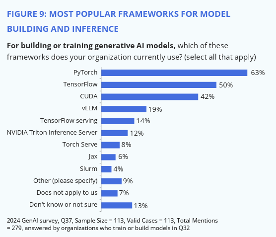
Regarding software for Deep Learning, the landscape is currently dominated by three software frameworks (listed in order of when they were published):


A detailed comparison of these frameworks is unnecessary. PyTorch and TensorFlow, being the oldest, have larger communities and comprehensive feature sets for both research and production. JAX, a newer framework, incorporates improvements over PyTorch and TensorFlow but is still evolving. Given their different programming paradigms (object-oriented vs. functional), a direct comparison is not particularly meaningful.
This course uses PyTorch due to its intuitive nature and its prevalence in our research. Currently, PyTorch is the dominant framework for published models, research papers, and competition winners.
The intention behind this set of exercises is to get everyone's PyTorch skills up to date. If you're already a PyTorch-Jedi, feel free to skip the first set of exercises, but I still recommend that you go through them. The exercises are in large part taken directly from the deep learning course at Udacity. Note that these exercises are given as notebooks, which is the only time we are going to use them actively in the course. Instead, after this set of exercises, we are going to focus on writing code in Python scripts.
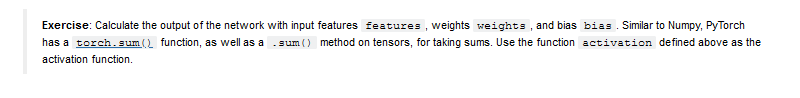
The notebooks contain a lot of explanatory text. The exercises that you are supposed to complete are inlined in the text in small "exercise" blocks:
For a refresher on deep learning topics, consult the relevant chapters in the deep learning book by Goodfellow, Bengio, and Courville (also available in the literature folder). While expertise in deep learning is not required to pass this course, a basic understanding of the concepts is beneficial. The course focuses on the software aspects of deploying deep learning models in production.
A note on installing Pytorch
Pytorch is a huge library with many dependencies. As writing this, if you naively install Pytorch like this
in a new virtual environment, this will result in a disk usage of around 6.6 GB! This is not a problem if you have to do it one time, but what you will experience throughout this course you will end up downloading and installing your project dependencies over and over again for different reasons (new virtual environments, containers, continuous integration systems etc.). For this reason, it is worth considering how you install Pytorch.
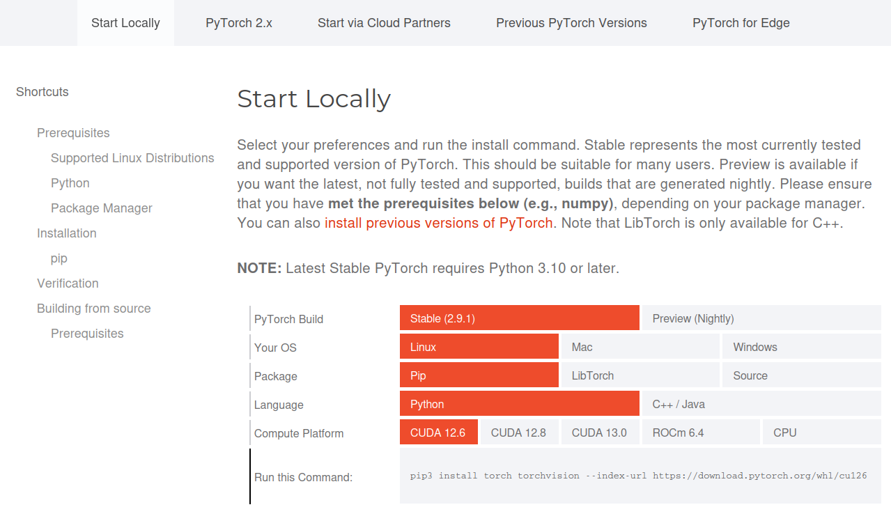
When naively installing Pytorch, you will fetch whatever build is available on PyPI which is most likely a GPU enabled build. But if you do not have a GPU in your computer, you should instead install the CPU only build. For comparison, the CPU only build of Pytorch is around 729 MB on disk. Usually, I always recommend going to Pytorch's homepage and use their selector to get the correct installation command for your system.
Here are some general installation commands for Pytorch:
For pip install you can basically follow the instructions on the Pytorch homepage. Here are some common
installation commands:
# CPU only
pip install torch torchvision torchaudio --index-url https://download.pytorch.org/whl/cpu
# GPU enabled
pip install torch torchvision --index-url https://download.pytorch.org/whl/cu126
If you want this to be part of your requirements.txt file, it needs to look something like this:
--index-url https://download.pytorch.org/whl/cu126
--extra-index-url https://pypi.org/simple

torch
# other dependencies
The reason we need both --index-url and --extra-index-url is that we need to force pip to look for Pytorch
packages in the Pytorch repository, but we also want to be able to install other packages from PyPI.
uv has dedicated a full page to installing Pytorch, which
I recommend you check out. Here is an example of how to configure your pyproject.toml file to install only CPU
version of Pytorch using uv:
❔ Exercises
Notebooks and uv
If you are using uv as your package manager, you may need to restart the Jupyter Notebook kernel after installing
new packages to ensure that the newly installed packages are recognized within the notebook environment.
-
Start a Jupyter Notebook session in your terminal (assuming you are at the root of the course material). Alternatively, you should be able to open the notebooks directly in your code editor. For VS Code users you can read more about how to work with Jupyter Notebooks in VS code in page from VScode documentation
-
Complete the Tensors in PyTorch notebook. It focuses on basic manipulation of PyTorch tensors. You can skip this notebook if you are comfortable doing this.
-
Complete the Neural Networks in PyTorch notebook. It focuses on building a very simple neural network using the PyTorch
nn.Moduleinterface. -
Complete the Training Neural Networks notebook. It focuses on how to write a simple training loop for training a neural network.
-
Complete the Fashion MNIST notebook, which summarizes concepts learned in notebooks 2 and 3 on building a neural network for classifying the Fashion MNIST dataset.
-
Complete the Inference and Validation notebook. This notebook adds important concepts on how to do inference and validation on our neural network.
-
Complete the Saving_and_Loading_Models notebook. This notebook addresses how to save and load model weights. This is important if you want to share a model with someone else.
🧠 Knowledge check
-
If tensor
ahas shape[N, d]and tensorbhas shape[M, d]how can we calculate the pairwise distance between rows inaandbwithout using a for loop?Solution
We can take advantage of broadcasting to do this
-
What should be the size of
Sfor an input image of size 1x28x28, and how many parameters does the neural network then have?from torch import nn neural_net = nn.Sequential( nn.Conv2d(1, 32, 3), nn.ReLU(), nn.Conv2d(32, 64, 3), nn.ReLU(), nn.Flatten(), nn.Linear(S, 10) )Solution
Since both convolutions have a kernel size of 3, stride 1 (default value) and no padding that means that we lose 2 pixels in each dimension, because the kernel cannot be centered on the edge pixels. Therefore, the output of the first convolution would be 32x26x26. The output of the second convolution would be 64x24x24. The size of
Smust therefore be64 * 24 * 24 = 36864. The number of parameters in a convolutional layer iskernel_size * kernel_size * in_channels * out_channels + out_channels(last term is the bias) and the number of parameters in a linear layer isin_features * out_features + out_features(last term is the bias). Therefore, the total number of parameters in the network is3*3*1*32 + 32 + 3*3*32*64 + 64 + 36864*10 + 10 = 387,466, which could be calculated by running: -
A working training loop in PyTorch should have these three function calls:
optimizer.zero_grad(),loss.backward(),optimizer.step(). Explain what would happen in the training loop (or implement it) if you forgot each of the function calls.Solution
optimizer.zero_grad()is in charge of zeroing the gradient. If this is not done, then gradients would accumulate over the steps, leading to exploding gradients.loss.backward()is in charge of calculating the gradients. If this is not done, then the gradients will not be calculated and the optimizer will not be able to update the weights.optimizer.step()is in charge of updating the weights. If this is not done, then the weights will not be updated and the model will not learn anything.
❔ Final exercise
As the final exercise, we will develop a simple baseline model that we will continue to develop during the course. For this exercise, we provide a corrupted subset of the MNIST dataset which can be downloaded from this Google Drive folder or using these two commands:
The data should be placed in a subfolder called data/corruptmnist in the root of the project. Your overall
task is the following:
Implement an MNIST neural network that achieves at least 85% accuracy on the test set.
Before any training can start, you should identify the corruption that we have applied to the MNIST dataset to create the corrupted version. This can help you identify what kind of neural network to use to get good performance, but any network should be able to achieve this.
One key point of this course is trying to stay organized. Spending time now organizing your code will save time in the future as you start to add more and more features. As subgoals, please complete the following exercises:
-
Implement your model in a script called
model.py.Starting point for
model.pySolution
The provided solution implements a convolutional neural network with 3 convolutional layers and a single fully connected layer. Because the MNIST dataset consists of images, we want an architecture that can take advantage of the spatial information in the images.
-
Implement your data setup in a script called
data.py. The data was saved usingtorch.save, so to load it you should usetorch.load.Saving the model
When saving the model, you should use
torch.save(model.state_dict(), "model.pt"), and when loading the model, you should usemodel.load_state_dict(torch.load("model.pt")). If you dotorch.save(model, "model.pt"), this can lead to problems when loading the model later on, as it will try to not only save the model weights but also the model definition. This can lead to problems if you change the model definition later (which you are most likely going to do).Starting point for
data.pySolution
Data is stored in
.ptfiles which can be loaded usingtorch.load(1). We iterate over the files, load them and concatenate them into a single tensor. In particular, we have highlighted the use of.unsqueezefunction. Convolutional neural networks (which we propose as a solution) need the data to be in the shape[N, C, H, W]whereNis the number of samples,Cis the number of channels,His the height of the image andWis the width of the image. The dataset is stored in the shape[N, H, W]and therefore we need to add a channel. The
The .ptfiles are nothing else than a.picklefile in disguise. Thetorch.save/torch.loadfunction is essentially a wrapper around thepicklemodule in Python, which produces serialized files. However, it is convention to use.ptto indicate that the file contains PyTorch tensors.
We have additionally in the solution added functionality for plotting the images together with the labels for inspection. Remember: all good machine learning starts with a good understanding of the data.
-
Implement training and evaluation of your model in the
main.pyscript. Themain.pyscript should be able to take additional subcommands indicating if the model is being trained or evaluated. It will look something like this:which can be implemented in various ways. We provide you with a starting script that uses the
typerlibrary to define a command line interface (CLI), which you can learn more about in this module later in the course.VS Code and command line arguments
If you try to execute the above code in VS Code using the debugger (F5) or the build run functionality in the upper right corner:
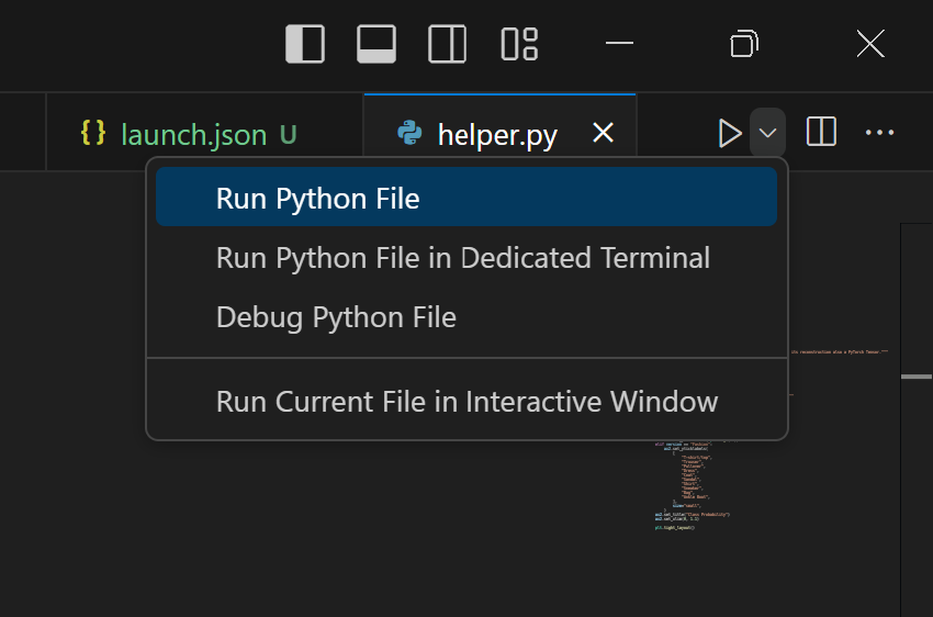
you will get an error message saying that you need to select a command to run e.g.
main.pyeither needs thetrainorevaluatecommand. This can be fixed by adding alaunch.jsonto a specialized.vscodefolder in the root of the project. Thelaunch.jsonfile should look something like this:{ "version": "0.2.0", "configurations": [ { "name": "Train", "type": "debugpy", "request": "launch", "program": "${file}", "args": [ "train", "--lr", "1e-4" ], "console": "integratedTerminal", "justMyCode": true } ] }This will inform VS Code that when we execute the current file (in this case
main.py), we want to run it with thetraincommand and additionally pass the--lrargument with the value1e-4. You can read more about creating alaunch.jsonfile here. If you want to have multiple configurations you can add them to theconfigurationslist as additional dictionaries.Starting point for
main.pySolution
The solution implements a simple training loop and evaluation loop. Furthermore, we have added additional hyperparameters that can be passed to the training loop. Highlighted in the solution are the different lines where we ensure that our model and data are moved to the GPU (or Apple MPS accelerator if you have a newer Mac) if available.
-
As documentation that your model is working when running the
traincommand, the script needs to produce a single plot with the training curve (training step vs. training loss). When theevaluatecommand is run, it should write the test set accuracy to the terminal.
It is part of the exercise not to implement this in notebooks, as code development in real life happens in scripts.
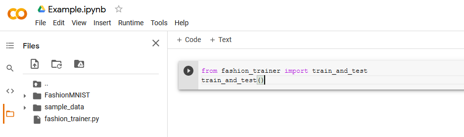
As the model is simple to run (for now), you should be able to complete the exercise on your laptop,
even if you are only training on CPU. That said, you are allowed to upload your scripts to your own "Google Drive" and
then you can call your scripts from a Google Colab notebook, which is shown in the image below where all code is
placed in the fashion_trainer.py script and the Colab notebook is just used to execute it.
Be sure to have completed the final exercise before the next session, as we will be building on top of the model you have created.