Scalable Inference

Inference is task of applying our trained model to some new and unseen data, often called prediction. Thus, scaling inference is different from scaling data loading and training, mainly due to inference normally only using a single data point (or a few). As we can neither parallelize the data loading or parallelize using multiple GPUs (at least not in any efficient way), this is of no use to us when we are doing inference. Secondly, inference is often not something we do on machines that can perform large computations, as most inference today is actually either done on edge devices e.g. mobile phones or in low-cost-low-compute cloud environments. Thus, we need to be smarter about how we scale inference than just throwing more compute at it.

In this module we are going to look at various ways that you can either reduce the size of your model and or make your model faster. Both are important for running inference fast regardless of the setup you are running your model on. We want to note that this is still very much an active area of research and therefore best practices for what to do in a specific situation can change.

Choosing the right architecture

Assume you are starting a completely new project and have to come up with a model architecture for doing this. What is you strategy? The common way to do this, is to look at prior work on similar problems that you are facing and either directly choosing the same architecture or creating some slight variation hereof. This is a great way to get started, but the architecture that you end up choosing may be optimal in terms of performance but not inference speed.

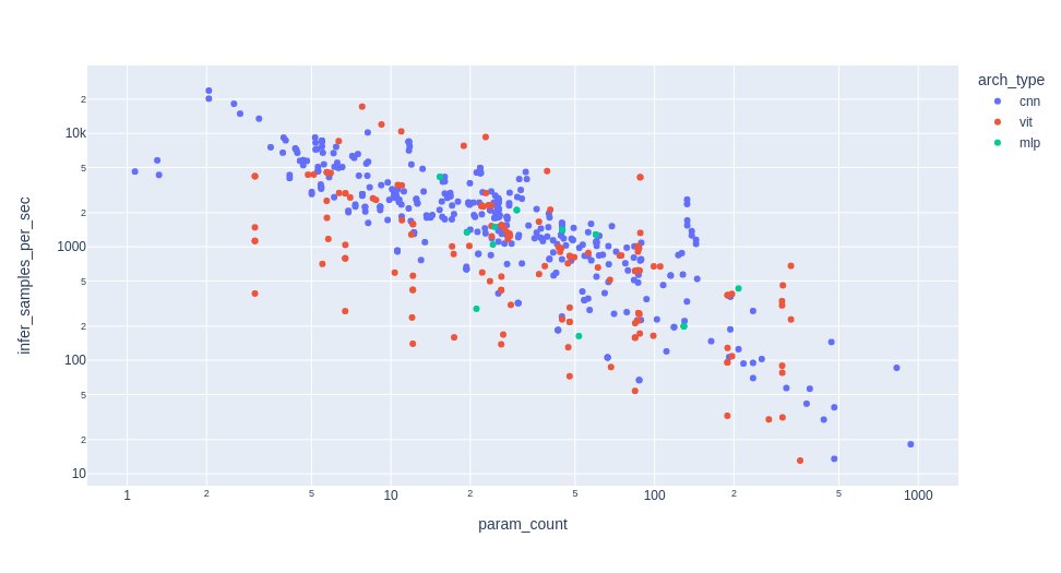
The fact is that not all base architectures are created equal, and a 10K parameter model with one architecture can have significantly different inference speed than another 10K parameter model with another architecture. For example, consider the figure below which compares a number of models from the [timm] package, colored based on their base architecture. The general trend is that the number of images that can be processed by a model per sec (y-axis) is inverse proportional to the number of parameters (x-axis). However, we in general see that convolutional base architectures (conv) are more efficient than transformer (vit) for the same parameter budget.

❔ Exercises

As dissed in this blogpost the largest increase in inference speed you will see (given some specific hardware) is choosing an efficient model architectures. In the exercises below we are going to investigate the inference speed of different architectures.

Start by checking out this table which contains a list of pretrained weights in torchvision. Try finding an
- Efficientnet
- Resnet
- Transformer based
model that have in the range of 20-30 mio parameters.

Write a small script that initialize all models and does inference with them. It should look something like this

import time
from torchvision import models

m1 = models.ModelArchitechture1()
m2 = models.ModelArchitechture2()
m3 = models.ModelArchitechture3()

input = torch.randn(100, 3, 256, 256)

for i, m in enumerate([m1, m2, m3]):
    tic = time.time()
    for _ in range(n_reps):
        _ = m(input)
    toc = time.time()
    print(f"Model {i} took: {(toc - tic) / n_reps}")

Does the results make sense? Based on the above figure we would expect that efficientnet is faster than resnet, which is faster than the transformer based model. Is this also what you are seeing?
To figure out why one net is more efficient than another we can try to count the operations each network need to do for inference. A operation here we can define as a FLOP (floating point operation) which is any mathematical operation (such as +, -, *, /) or assignment that involves floating-point numbers. Luckily for us someone has already created a python package for calculating this in pytorch: ptflops
1. Install the package
```
pip install ptflops
```
2. Try calling the get_model_complexity_info function from the ptflops package on the networks from the previous exercise. What are the results?
In the table from the initial exercise, you could also see the overall performance of each network on the Imagenet-1K dataset. Given this performance, the inference speed, the flops count what network would you choose to use in a production setting? Discuss when choosing one over another should be considered.

Quantization

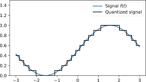
Quantization is a technique where all computations are performed with integers instead of floats. We are essentially taking all continuous signals and converting them into discretized signals.

As discussed in this blogpost series, while float (32-bit) is the primarily used precision in machine learning because is strikes a good balance between memory consumption, precision and computational requirement it does not mean that during inference we can take advantage of quantization to improve the speed of our model. For instance:

Floating-point computations are slower than integer operations
Recent hardware have specialized hardware for doing integer operations
Many neural networks are actually not bottlenecked by how many computations they need to do but by how fast we can transfer data e.g. the memory bandwidth and cache of your system is the limiting factor. Therefore working with 8-bit integers vs 32-bit floats means that we can approximately move data around 4 times as fast.
Storing models in integers instead of floats save us approximately 75% of the ram/harddisk space whenever we save a checkpoint. This is especially useful in relation to deploying models using docker (as you hopefully remember) as it will lower the size of our docker images.

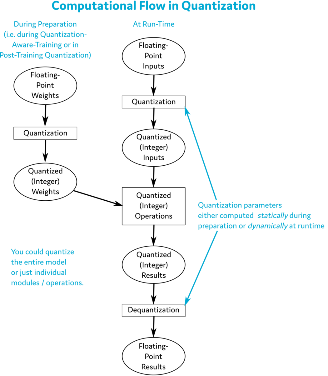
But how do we convert between floats and integers in quantization? In most cases we often use a linear affine quantization:

$$ x_{int} = \text{round}\left( \frac{x_{float}}{s} + z \right) $$

where $s$ is a scale and $z$ is the so called zero point. But how does to doing inference in a neural network. The figure below shows all the conversations that we need to make to our standard inference pipeline to actually do computations in quantized format.

❔ Exercises

Lets look at how quantized tensors look in Pytorch
1. Start by creating a tensor that contains both random numbers
2. Next call the torch.quantize_per_tensor function on the tensor. What does the quantized tensor look like? How does the values relate to the scale and zero_point arguments.
3. Finally, try to call the .dequantize() method on the tensor. Do you get a tensor back that is close to what you initially started out with.
As you hopefully saw in the first exercise we are going to perform a number of rounding errors when doing quantization and naively we would expect that this would accumulate and lead to a much worse model. However, in practice we observe that quantization still works, and we actually have a mathematically sound reason for this. Can you figure out why quantization still works with all the small rounding errors? HINT: it has to do with the central limit theorem
Lets move on to quantization of our model. Follow this tutorial from Pytorch on how to do quantization. The goal is to construct a model model_fc32 that works on normal floats and a quantized version model_int8. For simplicity you can just use one of the models from the tutorial.
Lets try to benchmark our quantized model and see if all the trouble that we went through actually paid of. Also try to perform the benchmark on the non-quantized model and see if you get a difference. If you do not get an improvement, explain why that may be.

Pruning

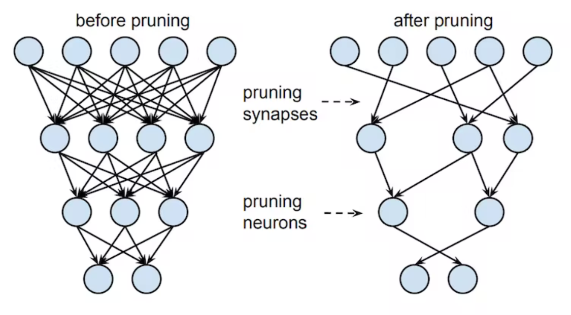
Pruning is another way for reducing the model size and maybe improve performance of our network. As the figure below illustrates, in pruning we are simply removing weights in our network that we do not consider important for the task at hand. By removing, we here mean that the weight gets set to 0. There are many ways to determine if a weight is important but the general rule that the importance of a weight is proportional to the magnitude of a given weight. This makes intuitively sense, since weights in all linear operations (fully connected or convolutional) are always multiplied onto the incoming value, thus a small weight means a small outgoing activation.

❔ Exercises

We provide a start script that implements the famous LeNet in this file. Open and run it just to make sure that you know the network.
Pytorch have already some pruning methods implemented in its package. Import the prune module from torch.nn.utils in the script.
Try to prune the weights of the first convolutional layer by calling
```
prune.random_unstructured(module_1, name="weight", amount=0.3)  # (1)!
```
1. You can read about the prune method here.
Try printing the named_parameters, named_buffers before and after the module is pruned. Can you explain the difference and what is the connection to the module_1.weight attribute.
Try pruning the bias of the same module this time using the l1_unstructured function from the pruning module. Again check the named_parameters, named_buffers argument to make sure you understand the difference between L1 pruning and unstructured pruning.
Instead of pruning only a single module in the model lets try pruning the whole model. To do this we just need to iterate over all named_modules in the model like this:
```
for name, module in new_model.named_modules():
    prune.l1_unstructured(module, name='weight', amount=0.2)
```
But what if we wanted to apply different pruning to different layers. Implement a pruning scheme where
- The weights of convolutional layers are L1 pruned with amount=0.2
- The weights of linear layers are unstructured pruned with amount=0.4
Print print(dict(new_model.named_buffers()).keys()) after the pruning to confirm that all weights have been correctly pruned.
The pruning we have looked at until know have only been local in nature e.g. we have applied the pruning independently for each layer, not accounting globally for how much we should actually prune. As you may realize this can quickly lead to an network that is pruned too much. Instead, the more common approach is too prune globally where we remove the smallest X amount of connections:
1. Start by creating a tuple over all the weights with the following format
```
parameters_to_prune = (
    (model.conv1, 'weight'),
    # fill in the rest of the modules yourself
    (model.fc3, 'weight'),
)
```
  The tuple needs to have length 5. Challenge: Can you construct the tuple using for loops, such that the code works for arbitrary size networks?
2. Next prune using the global_unstructured function to globally prune the tuple of parameters
```
prune.global_unstructured(
    parameters_to_prune,
    pruning_method=prune.L1Unstructured,
    amount=0.2,
)
```
3. Check that the amount that have been pruned is actually equal to the 20% specified in the pruning. We provide the following function that for a given submodule (for example model.conv1) computes the amount of pruned weights
```
def check_prune_level(module: nn.Module):
    sparsity_level = 100 * float(torch.sum(module.weight == 0) / module.weight.numel())
    print(f"Sparsity level of module {sparsity_level}")
```
With a pruned network we really want to see if all our effort actually ended up with a network that is faster and/or smaller in memory. Do the following to the globally pruned network from the previous exercises:
1. First we need to make the pruning of our network permanent. Right now it is only semi-permanent as we are still keeping a copy of the original weights in memory. Make the change permanent by calling prune.remove on every pruned module in the model. Hint: iterate over the parameters_to_prune tuple.
2. Next try to measure the time of a single inference (repeated 100 times) for both the pruned and non-pruned network
```
import time
tic = time.time()
for _ in range(100):
    _ = network(torch.randn(100, 1, 28, 28))
toc = time.time()
print(toc - tic)
```
  Is the pruned network actually faster? If not can you explain why?
3. Next lets measure the size of our network (called pruned_network) and a freshly initialized network (called network):
```
torch.save(pruned_network.state_dict(), 'pruned_network.pt')
torch.save(network.state_dict(), 'network.pt')
```
  Lookup the size of each file. Are the pruned network actually smaller? If not can you explain why?
4. Repeat the last exercise, but this time start by converting all pruned weights to sparse format first by calling the .to_sparse() method on each pruned weight. Is the saved model smaller now?

This ends the exercises on pruning. As you probably realized in the last couple of exercises, then pruning does not guarantee speedups out of the box. This is because linear operations in Pytorch does not handle sparse structures out of the box. To actually get speedups we would need to deep dive into the sparse tensor operations, which again does not even guarantee that a speedup because the performance of these operations depends on the sparsity structure of the pruned weights. Investigating this is out of scope for these exercises, but we highly recommend checking it out if you are interested in sparse networks.

Knowledge distillation

Knowledge distillation is somewhat similar to pruning, in the sense that it tries to find a smaller model that can perform equally well as a large model, however it does so in a completely different way. Knowledge distillation is a model compression technique that builds on the work of Bucila et al. in which we try do distill/compress the knowledge of a large complex model (also called the teacher model) into a simpler model (also called the student model).

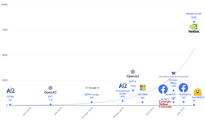
The best known example of this is the DistilBERT model. The DistilBERT model is a smaller version of the large natural-language procession model Bert, which achieves 97% of the performance of Bert while only containing 40% of the weights and being 60% faster. You can see in the figure below how it is much smaller in size compared to other models developed at the same time.

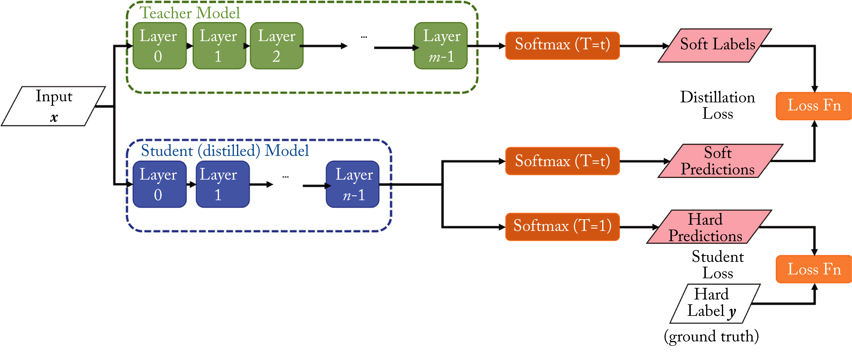
Knowledge distillation works by assuming we have a big teacher that is already performing well that we want to compress. By running our training set through our large model we get a softmax distribution for each and every training sample. The goal of the students, is to both match the original labels of the training data but also match the softmax distribution of the teacher model. The intuition behind doing this, is that teacher model needs to be more complex to learn the complex inter-class relasionship from just (one-hot) labels. The student on the other hand gets directly feed with softmax distributions from the teacher that explicit encodes this inter-class relasionship and thus does not need the same capasity to learn the same as the teacher.

❔ Exercises

Lets try implementing model distillation ourself. We are going to see if we can achieve this on the cifar10 dataset. Do note that exercise below can take quite long time to finish because it involves training multiple networks and therefore involve some waiting.

Start by install the transformers and datasets packages from Huggingface
```
pip install transformers
pip install datasets
```
which we are going to download the cifar10 dataset and a teacher model.

Next download the cifar10 dataset

from datasets import load_dataset
dataset = load_dataset("cifar10")

Next lets initialize our teacher model. For this we consider a large transformer based model:

from transformers import AutoFeatureExtractor, AutoModelForImageClassification
extractor = AutoFeatureExtractor.from_pretrained("aaraki/vit-base-patch16-224-in21k-finetuned-cifar10")
model = AutoModelForImageClassification.from_pretrained("aaraki/vit-base-patch16-224-in21k-finetuned-cifar10")

To get the logits (un-normalized softmax scores) from our teacher model for a single datapoint from the training dataset you would extract it like this:

sample_img = dataset['train'][0]['img']
preprocessed_img = extractor(dataset['train'][0]['img'], return_tensors='pt')
output =  model(**preprocessed_img)
print(output.logits)
# tensor([[ 3.3682, -0.3160, -0.2798, -0.5006, -0.5529, -0.5625, -0.6144, -0.4671, 0.2807, -0.3066]])

Repeat this process for the whole training dataset and store the result somewhere.

Implement a simple convolutional model. You can create a custom one yourself or use a small one from torchvision.
Train the model on cifar10 to convergence, so you have a base result on how the model is performing.

Redo the training, but this time add knowledge distillation to your training objective. It should look like this:

for batch in dataset:
    # ...
    img, target, teacher_logits = batch
    preds = model(img)
    loss = torch.nn.functional.cross_entropy(preds, target)
    loss_teacher = torch.nn.functional.cross_entropy(preds, teacher_logits)
    loss = loss + loss_teacher
    loss.backward()
    # ...

Compare the final performance obtained with and without knowledge distillation. Did the performance improve or not?

This ends the module on scaling inference in machine learning models.